SOS Plugin
Requirements | Change log | Screenshots | Parameters | Outputs | Description and Video tutorials
This is a set of plugins for single molecule analysis and localization that were developed and published together with the paper:
 |
M. Reuter, A. Zelensky, I. Smal, E. Meijering, W. A. van Cappellen, H. M. de Gruiter, G. J. van Belle, M. E. van Royen, A. B. Houtsmuller, J. Essers, R. Kanaar, C. Wyman, BRCA2 diffuses as oligomeric clusters with RAD51 and changes mobility after DNA damage in live cells, Journal of Cell Biology, 207(5):599-613, 2014 |
It can be used to detect spot-like objects by fitting a Gaussian PSF into intensity profiles, and then either to group the detection from different frames (into “molecules”/clusters) or to perform simple (nearest-neighbor) tracking (more advanced tracking/linking methods will be added later).
This plugin also participated in “Single Molecule Localization Microscopy” Challenge, at ISBI 2013 (link).
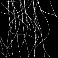
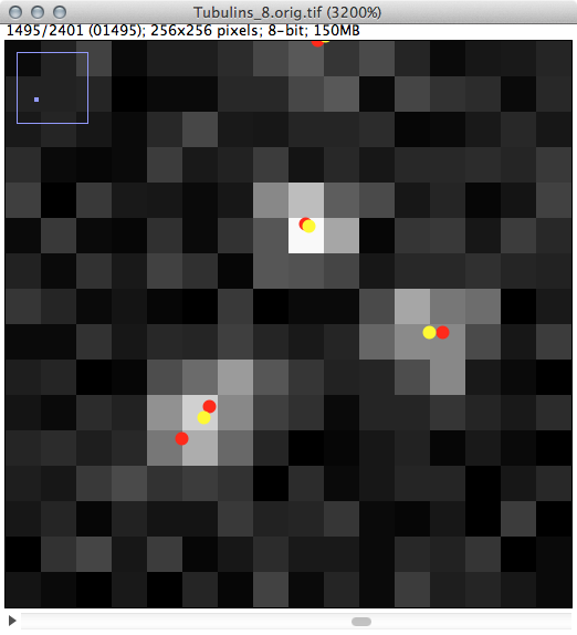
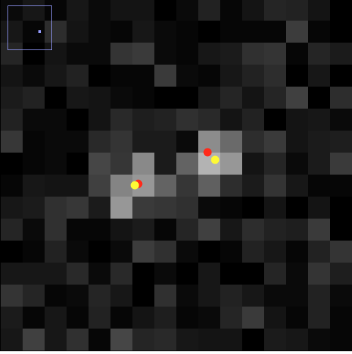
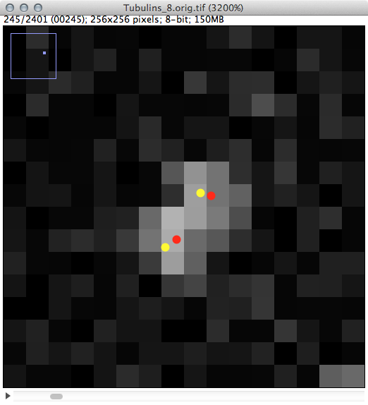
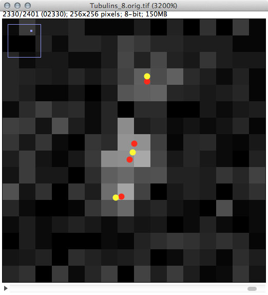
Above, the results of fitting a mixture of PSFs into a blobby intensity profiles (red – ground truth positions, yellow – results of mixture fitting).
If you use these plugins in your analysis, please reference the article mentioned above.
- SOS Plugin
- Test dataset testImage1.zip (image and parameters.txt)
- Test dataset testImage2.zip (image and parameters.txt)
Requirements
The following libraries should be downloaded and placed in the ImageJ’s plugins folder:
- MTrackJ_.jar
- imagescience.jar
- Jama-1.0.2.jar or download from the official website
Change log
- 05-02-2015 v2.0.3 – spot intensity values are now re-estimated after estimation of position and sigma, so the final intensity values not necessary integers
- 02-02-2015 v2.0.2 – added drift correction procedure (see below)
- 13-01-2015 v2.0.1 – removed color indicators in the dialogs, in order to make it compatible with OpenJDK
- 04-12-2014 v2.0.0 – initial public release
Screenshots
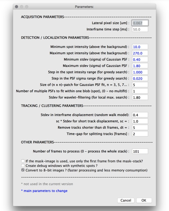
Parameters (as in the parameters.txt file)
| Parameter | Description |
|---|---|
| dx | lateral pixel size (not used in the current version) |
| dt | sampling time (not used in the current version) |
| sigma_D | stdev in the nearest-neighbor motion model, during the tracking/clustering, a detection from one time frame is linked to the detection in the next frame if the spatial distance between those two detections is less than 3*sigma_D |
| stdev_scale | scaling of the sigmaD for tracks that are broken for many time points. If a track has a ‘gap’ of several time frames, (so consists of two sub-tracks), those sub-tracks are connected into one tracks if the spatial distance between the ‘head’ of one sub-track and the ‘tail’ of the other is less than 3 * stdev_scale * sigma_D, otherwise those two su-tracks are considered as separate tracks. |
| I_min | minimum spot intensity, above a local background (which is automatically estimated) |
| I_max | maximum spot intensity, above a local background (which is automatically estimated) |
| s_min | minimum stdev of the Gaussian (PSF) that is going to be fitted |
| s_max | maximum stdev of the Gaussian (PSF) that is going to be fitted |
| T_max | number of frames to process. (0 – means ‘process all frames’ |
| masksize | mask size for Gaussian (PSF) fit. The size of the image patch/support for a Gaussian fit, which is of order 5*sigma-by-5*sigma, and should be given as integer, odd number. For example, 3 or 5 would correspond to 3×3 and 5×5 patches, which are good for fitting PSFs with sigma ~ 0.5-1.5 pixels. |
| binning | binning of the origin image (not used anymore). In the current version this parameter is used for fitting multiple Gaussian PSF models in one intensity blobs. The value 0 here means that no multi-fit will be performed, which is equal to doing multi-fit with 1 Gaussian PSF. |
| gaussianFilteringStdev | prefiltering of the image in order to get rid of many local maxima (Gauss stdev)(not used anymore), instead this parameter now is the threshold for the wavelet coefficients, w_th=gaussianFilteringStdev*w_stdev, with reasonable values in the range of 1.5-3 (which corresponds to the thresholing with some of false positives) |
| isUseFirstMaskFrame | if the mask file (stack with “binary” images exists, use all the frames or only the first one. Here, “binary” means that even if 8bit or 16 bit grayscale image is provided, all zero pixel values are considered as 0, and all non-zero values are 1). |
| isCreateDebugOutput | should the debug output images be created |
| deltaT | tracks shorter than deltaT will be discarded |
| gapT | if the gap of more than gapT frames exists in a track, split that track in several tracks |
| step_dI | step for tabulation of the intensity range between I_min and I_max. Reasonable walues are 1 for 8 bit images, and 10-100 for 16bit images |
| step_dS | step for tabulation of the sigma range between s_min and s_max. Reasonable values are (s_max-s_min)/100 |
Outputs
The following files are stored in the working directory as outputs in the form of simple text files:detections.txt
| x | y | frame numb. | intensity | sigma | fit error | stdev in x | stdev in y | stdev in intensity | stdev in sigma |
|---|---|---|---|---|---|---|---|---|---|
| .. | .. | .. | .. | .. | .. | .. | .. | .. | .. |
detections.filtered.txt
| x | y | frame numb. | intensity | sigma | fit error | stdev in x | stdev in y | stdev in intensity | stdev in sigma |
|---|---|---|---|---|---|---|---|---|---|
| .. | .. | .. | .. | .. | .. | .. | .. | .. | .. |
tracks.simple.txt or clusters.simple.txt
| x | y | track id | existence | intensity | sigma | not used |
|---|---|---|---|---|---|---|
| .. | .. | .. | 0/1 | .. | .. | .. |
tracks.simple.filtered.txt or clusters.simple.filtered.txt
| t | x | y | track id | displacement from the previous time point | intensity | sigma | fit error |
|---|---|---|---|---|---|---|---|
| .. | .. | .. | .. | -1 (if the first point of the track) | .. | .. | .. |
tracks.simple.diff.txt
| track id | k (as in MSD(k)) | MSD(k) | number of counts that contributed |
|---|---|---|---|
| .. | .. | .. | .. |
results.track.intensity.txt or results.cluster.intensity.txt
| track intensity | stdev in track intensity | number of detections, forming the track |
|---|---|---|
| .. | .. | .. |
results.track.length.txt or results.cluster.length.txt
| track length |
|---|
| .. |
Description of Plugins
SM PrepareData (video tutorials: link 1, link 2)
- Prepare the input image data (image or stack) for other plugins
- Input: either a single frame or image stack, opened in ImageJ
- Output: a new folder at the location of the opened image (further referenced as WORK_DIR), which contains the properly adjusted tif file (e.g. 8-bit, z-slices are arranged as time frames) and parameter file “parameters.txt”
SM PrepareData (BATCH) (video tutorials: link 1, link 2)
- The same as above, but for multiple image files. The same parameter file will be written to multiple folders.
- Input: Selection of multiple tif-files using a file dialog (with Ctrl or Command keys)
- Output: Multiple folders in the same place where the input image files are located, containing the adjusted tif-files and parameter files
SM Create Mask From ROI (video tutorials: link 1, link 2)
- Create a binary mask, which will be used to perform the object localization and detection only within the specified (by the mask) regions. Here, “binary” means that even if 8bit or 16 bit grayscale image is provided, all zero pixel values are considered as 0, and all non-zero values are 1).
- Input: Opened in ImageJ image.
- How to run: Select any ROI-tool from ImageJ, draw a ROI, add it to the ROI Manager, draw and add more ROIs if desired, and then run the plugin from the menu.
- Output: 8-bit image “mask.tif” which should be saved manually to WORK_DIR.
SM Gauss Fit (video tutorials: link 1, link 2)
- Main plugin that does Gaussian PSF fitting
- Input: Image sequence as one tif-file (should be opened with ImageJ before processing, for example from the WORK_DIR), where the “number of frames” property in ImageJ (ImageJ’s Menu->Image->Properties…) reflects the number of frames in the sequence, and “number of Z-slices” property is set to 1. The other required file is parameters.txt in the same folder (e.g. WORK_DIR), where the tif-file is located.
- Output: detections in the text file detections.txt (in WORK_DIR) and the same information in the .mdf format in order to visualize in MTrackJ
SM Gauss Fit (BATCH) (video tutorials: link 1, link 2)
- Does the same job as “SM Gauss Fit” but for multiple files (batch mode)
- Input: folders selected using the file-dialog (multiple folders can be selected with Ctrl or Command keys), which contain the tif-tiles
- Output: the results of detection and tracking/clustering, which are stored in the corresponding WORK_DIR
- Macro usage: run(“SM Gauss Fit (BATCH)”, “imagefolder=’/Users/ssss/data/aaaa/frap 12′ dotracking=false doclustering=true dodetection=true uselut=true usemultithreading=true”);
- Macro usage: run(“SOS (batch multithread)”, “imagefolder=’/Users/ssss/data/aaaa/frap 12′ dotracking=false doclustering=true dodetection=true”);
SM Gauss Fit (multithread and mixture) (video tutorials: link 1, link 2)
- Main plugin that does Gaussian PSF fitting but using the Java multithreading (proportionally faster on multicore CPUs) and performs fitting of multiple Gaussian PSFs. The image intensity regions at the local maxima, where fitting of a single PSF led to the estimated sigma in the interval [sigma_max – 0.1, sigma_max], are re-fitted using a mixture of M Gaussian PSFs (M is specified in the dialog and corresponds to the maximum number of components that will be used. Some components of the mixture can converge to the same local maxima, so the final number of estimated mixtures is always between 1 and M)
- Input: Image sequence specified using a file-open dialog. The other required file is parameters.txt in the same folder (e.g. WORK_DIR), where the tif-file is located.
- Output: detections in the text file detections.txt (in WORK_DIR) and the same information in the .mdf format in order to visualize in MTrackJ
SM Gauss Fit (multithread and mixture, BATCH)
- Does the same job as “SM Gauss Fit (multithread and mixture)” but for multiple files (batch mode)
- Input: folders, selected using a file-dialog (multiple folders can be selected with Ctrl or Command keys), which contain the tif-tiles
- Output: the results of detection and tracking/clustering, which are stored in the corresponding WORK_DIR
SM Filter Results using Thresholds (video tutorials: link 1, link 2)
- Thresholds/filters the detections from detections.txt file using basic thresholds for intensity and stdev (sigma) of the Gaussian PSF fit
- Input: Image of interest should be opened beforehand (from WORK_DIR)
- Output: after the thresholds are applied, the new detections are saved into detections.filtered.txt together with the corresponding detections.filtered.txt.mdf file (to WORK_DIR)
- Macro usage: run(“SM Filter Results using Thresholds”, “intensity_min=30 intensity_max=30 sigma_min=0.30 sigma_max=1.30”);
SM Create Parameter Histogram (video tutorials: link 1, link 2)
- Builds a 2D histogram of spot intensity (y-axis) vs stdev (Gaussian PSF sigma) (x-axis). The actual values of the intensity and stdev can be seen while going with the mouse pointer over the histogram image and noticing the values “x=…” and “y=…” in the ImageJ status bar.
- Input: Asks for the main image sequence (from WORK_DIR)
- Output: Saves the histogram into parameters.histogram.tif (into WORK_DIR)
SM Filter Results using ROI (video tutorials: link 1, link 2)
- Selects a ROI-like threshold in the parameter histogram and applies them to detections.txt
- Input: Both the original sequence and parameters.histogram.tif should be opened. Then ROI (box, oval, or freehand) should be drawn (in the histogram image) and added to the ROI manager. After that this plugin can be run.
- Output: detections.filtered.txt and .mdf with applied ROI thresholds (saved into WORK_DIR).
SM Simple Tracking (video tutorials: link 1, link 2)
- Performs tracking (linking of the detected objects into tracks) on a basis of nearest neighbor (the position of the object in the current frame is used to look for the nearest neighbor in the next frame)
- Input: Image of interest should be opened beforehand (from WORK_DIR) and the SM Gauss Fit should be run beforehand (so the detections.txt file should exist in that folder)
- Output: files such as tracks.simple.txt as well as lots of plots
- Macro Usage: run(“SM Simple Tracking”, “detections_name=detections.drift-corrected.txt“);
SM Simple Clustering
- Performs clustering (linking of the detected objects into clusters) on a basis of nearest neighbor (the average position of the objects in the previous frames (the position of the cluster) is used to look for the nearest neighbor in the next frame)
- Input: Image of interest should be opened beforehand (from WORK_DIR) and the SM Gauss Fit should be run beforehand (so the detections.txt file should exist in that folder)
- Output: files such as clusters.simple.txt as well as lots of plots
- Macro Usage: run(“SM Simple Clustering”, “detections_name=detections.drift-corrected.txt”);
SM Drift Correction
- Performs drift correction using displacement information from, for example, beads or other markers.
- Input: the SM Gauss Fit procedure should be run using additionally ‘mask-control.tif’ image, which is a binary (in ImageJ, for 8bit or 16bit images, the pixel values of 0 will be considered as “0” and non-zero pixels as “1”) mask, indicating the regions, where the beads or other markers are located. That mask image should be placed in WORK_DIR. The output will consist of two files ‘detections.txt’ and ‘detections.mask-control.txt’ which contain detections of spots and detections of beads, respectively.
- Output: ‘detections.mask-control.txt’ is used to compute the drift displacements, which are saved to ‘drift.mask-control.txt, and applied to original ‘detections.txt’ to produce ‘detections.drift-corrected.txt’. Then, the linking (using Simple Tracking or Clustering can be used. In order to do that, file ‘detections.drift-corrected.txt’ needs to be renamed back to ‘detections.txt’